Neural Style Transfer Part 1 : Introduction
Neural Style Transfer was first published in the paper “A Neural Algorithm of Artistic Style” by Gatys et al., originally released in 2015. It is an image transformation technique which modifies one image in the style of another image.
If these line do not convince you then see the images below,
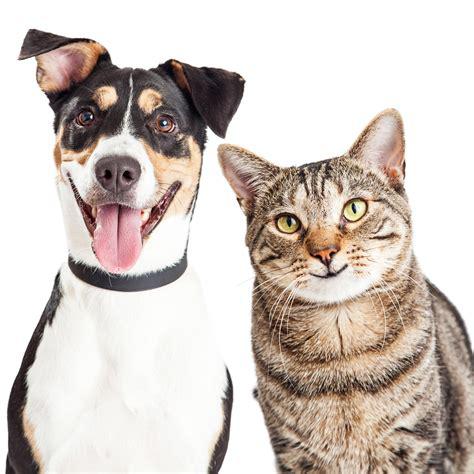
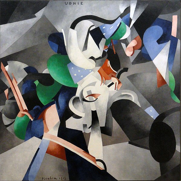
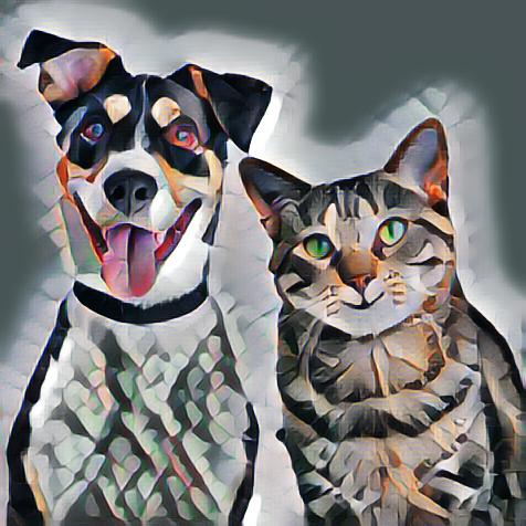
here we have two images one shows the cute friendship of cat and dog while other is udnie painting by Francis Picabia. Using style transfer technique we have modified friendship image in the style of udnie painting, now it looks like an impressive artwork. If this motivates you and wants to know how this works and how to do this with your images then continue reading I am going to explain this.
I am dividing this tutorial into two parts:
-
In the first part, we are tackling some theory and implementing Gatys style transfer which was originally released in 2015 by Gatys et al. But generating an image using this technique takes time which depends on compute power provided. In my system it takes about 10 min for an image because of this we would not like to use this for styling videos.
-
In the second part, we will implement another variant of style transfer which we can call fast style transfer. It was proposed in this paper by Justin Johnson. This is hundreds of times faster than gatys style transfer. It is so fast that we can use this in realtime videos too.
We have used convolutional networks for image classifications and detection problems in machine learning many times but this time we are using them for style transfer. Implementing this on my own helps me to evolve in deep learning. I was using keras before and trapped inside using fit method and sequential model for all image tasks. But implementing this helps me to break that trap and deep dive inside model architecture, loss function and training loop. This skill also helps to understand and implement different model architectures on my own from research papers. I hope it will help you too.
Before starting the tutorial note:
Content Image: The image which we want to stylize.Style Image: The image whose style we want to embed in our content image.Output Image: The output styled image, we will be optimizing this image(more details later) to create a styled image.
Steps to create style transfer
- first, we will define our content image and style image using which we will generate an output image
- we are using a pre-trained model which will provide us feature maps at different layers. Now the question may arise why the need of these activations? In style transfer, we want the content of content image and style(textures) of style image in our output image. There is no direct way to calculate content and style of an image, Since convolutional feature maps capture a good representation of features of images we will use these feature maps from Conv net to calculate them(the process of calculating this is explained later in the post).
- we extract feature maps for style, content and output image, and use these maps to calculate a loss value(loss function explained later)
- The loss we calculated is then used to optimize our output image and create the styled image.
1
2
content_img_path = "starry_nights.jpg"
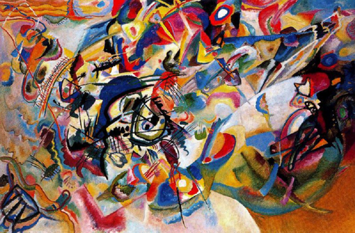
style_img_path = "vassily_kandinsky.jpg"
We start by defining the path to our style and content images. We are using starry image painting as a content image and Vassily Kandinsky painting as style.
1
2
3
4
5
6
7
8
import numpy as np
import tensorflow as tf
from tensorflow.keras.applications import vgg19
from tensorflow.keras.models import load_model, Model
from PIL import Image
import time
import IPython.display as display
from tqdm.notebook import tqdm
Next, we import all required modules which we will use:
numpy: for arrays manipulationtensorflow: for tensor operationstensorflow.keras: high-level neural network library for tensorflow for creating neural networkspillow: for converting an image to numpy array and numpy array to image, saving out output image.time: for calculating the time of each iterationIpython.display: for displaying images in notebooktqdm: for graphical counters
1
2
3
4
5
6
7
8
def load_image(image_path,max_dim=512):
    img = Image.open(image_path)
    img = img.convert("RGB")
    img.thumbnail([max_dim,max_dim])
    img = np.array(img,dtype=np.float32)
    img = img / 255.0
    img = np.expand_dims(img,axis=0)
    return img
the above function
- loads image from the path
- convert it into RGB format
- resize it with max dimension specified while maintaining aspect ratio
- converting an image to numpy array and creating a batch of a single image since neural networks expects the input to be in batches.
1
2
3
def deprocess_image(img):
    img = 255*img
    return np.array(img, np.uint8)
This function will scale image pixels from range [0, 1] to range [0, 255]
1
2
3
4
5
6
7
def array_to_img(array, deprocessing=False):
    if deprocessing:
        array=deprocess_image(array)
    if np.ndim(array)>3:
        assert array.shape[0]==1
        array=array[0]
    return Image.fromarray(array)
the above function will convert an array to an image. if deprocessing is true it will first deprocess vgg preprocessing and then convert array to image
1
2
3
def show_image(img, deprocessing=True):
    image=array_to_img(img, deprocessing)
    display.display(image)
the above function will show image in the notebook by first converting the array to image
1
2
3
content_image = load_image(content_img_path)
print(content_image.shape)
show_image(content_image)
(1, 300, 454, 3)

Now, let us load our content image and display it.
1
2
3
style_image = load_image(style_img_path)
print(style_image.shape)
show_image(style_image)
(1, 336, 512, 3)
Similarly, load style image and display it.
1
2
3
4
5
def stylized_model(model, layer_names):
    model.trainable=False
    outputs=[model.get_layer(name).output for name in layer_names]
    new_model=Model(inputs=model.input,outputs=outputs)
    return new_model
the above function creates a stylized model. Since we are not training our model so we set trainable to false. Our stylized model takes input as an image and outputs the activations of layers which we will use to extract content and style from the image. This function takes:
- pre-trained model which we will use to extract features from images (we are using vgg pre-trained model as it was used in original implementation).
- layer names from which we want to extract features
1
2
vgg=vgg19.VGG19(weights='imagenet',include_top=False)
vgg.summary()
Model: "vgg19"
_________________________________________________________________
Layer (type)                 Output Shape              Param #
=================================================================
input_1 (InputLayer)         [(None, None, None, 3)]   0
_________________________________________________________________
block1_conv1 (Conv2D)        (None, None, None, 64)    1792
_________________________________________________________________
block1_conv2 (Conv2D)        (None, None, None, 64)    36928
_________________________________________________________________
block1_pool (MaxPooling2D)   (None, None, None, 64)    0
_________________________________________________________________
block2_conv1 (Conv2D)        (None, None, None, 128)   73856
_________________________________________________________________
block2_conv2 (Conv2D)        (None, None, None, 128)   147584
_________________________________________________________________
block2_pool (MaxPooling2D)   (None, None, None, 128)   0
_________________________________________________________________
block3_conv1 (Conv2D)        (None, None, None, 256)   295168
_________________________________________________________________
block3_conv2 (Conv2D)        (None, None, None, 256)   590080
_________________________________________________________________
block3_conv3 (Conv2D)        (None, None, None, 256)   590080
_________________________________________________________________
block3_conv4 (Conv2D)        (None, None, None, 256)   590080
_________________________________________________________________
block3_pool (MaxPooling2D)   (None, None, None, 256)   0
_________________________________________________________________
block4_conv1 (Conv2D)        (None, None, None, 512)   1180160
_________________________________________________________________
block4_conv2 (Conv2D)        (None, None, None, 512)   2359808
_________________________________________________________________
block4_conv3 (Conv2D)        (None, None, None, 512)   2359808
_________________________________________________________________
block4_conv4 (Conv2D)        (None, None, None, 512)   2359808
_________________________________________________________________
block4_pool (MaxPooling2D)   (None, None, None, 512)   0
_________________________________________________________________
block5_conv1 (Conv2D)        (None, None, None, 512)   2359808
_________________________________________________________________
block5_conv2 (Conv2D)        (None, None, None, 512)   2359808
_________________________________________________________________
block5_conv3 (Conv2D)        (None, None, None, 512)   2359808
_________________________________________________________________
block5_conv4 (Conv2D)        (None, None, None, 512)   2359808
_________________________________________________________________
block5_pool (MaxPooling2D)   (None, None, None, 512)   0
=================================================================
Total params: 20,024,384
Trainable params: 20,024,384
Non-trainable params: 0
_________________________________________________________________
Here we initiate pre-trained vgg19 network (vgg network with 19 blocks) without its final classification dense layers as we only need its feature extractor and then we print its model summary.
1
2
3
4
5
6
7
8
9
## style and content layers

content_layers=['block5_conv2']

style_layers=['block1_conv1',
             'block2_conv1',
             'block3_conv1',
             'block4_conv1',
             'block5_conv1']
Let’s define layers from which we want to extract features for style and content images. We try to extract the appearance of our style image from all scenarios extracted by conv nets, so we have used multiple blocks of conv layers to capture feature maps at different spatial scales.
- We have used higher conv layer as a content layer because higher convolutional layers have learned complex and high-level features
- For style layers, we have used various layers at different scales to capture feature maps at different spatial scales.
1
2
content_model = stylized_model(vgg, content_layers)
style_model = stylized_model(vgg, style_layers)
Here we initiate two models with content layers (content_model) and style_layers (style_model) just to check how we are getting outputs from these models.
1
2
3
4
content_outputs = content_model(content_image)
for layer_name, outputs in zip(content_layers, content_outputs):
    print(layer_name)
    print(outputs.shape)
block5_conv2
(18, 28, 512)
We get output from a layer which we defined in content_layers list. The output is a feature map spit out by conv layer (block5_conv2) of shape (18,28,512)
1
2
3
4
style_outputs = style_model(style_image)
for layer_name,outputs in zip(style_layers, style_outputs):
    print(layer_name)
    print(outputs.shape)
block1_conv1
(1, 336, 512, 64)
block2_conv1
(1, 168, 256, 128)
block3_conv1
(1, 84, 128, 256)
block4_conv1
(1, 42, 64, 512)
block5_conv1
(1, 21, 32, 512)
Similarly, we can check output feature maps from layers defined in style_layers list
1
model = stylized_model(vgg, style_layers + content_layers)
Now let’s create a model which we will be used for style transfer. We create a vgg model which outputs all feature maps from the layers defined in style_layers and content_layers when an image is passed through it.
1
2
3
4
5
6
7
8
9
def get_output_dict(model, inputs):
    inputs = inputs*255.0
    preprocessed_input = vgg19.preprocess_input(inputs)
    style_length = len(style_layers)
    outputs = model(preprocessed_input)
    style_output,content_output = outputs[:style_length],outputs[style_length:]
    content_dict = {name:value for name,value in zip(content_layers,content_output)}
    style_dict = {name:value for name,value in zip(style_layers,style_output)}
    return {'content':content_dict,'style':style_dict}
The above function takes style transfer model and image as input and spits out output feature maps for content and style layers in a python dictionary.
This dictionary has 2 keys:
- content: has all feature maps for the image from content_layers
- style: has all feature maps for the image from style_layers
1
2
3
4
5
6
7
8
9
10
results = get_output_dict(model, style_image)

print("Content Image output Feature maps: ")
for layer_name,output in sorted(results['content'].items()):
    print(layer_name)
    print(output.shape)

for layer_name,output in sorted(results['style'].items()):
    print(layer_name)
    print(output.shape)
Content Image output Feature maps:
block5_conv2
(1, 21, 32, 512)
block1_conv1
(1, 336, 512, 64)
block2_conv1
(1, 168, 256, 128)
block3_conv1
(1, 84, 128, 256)
block4_conv1
(1, 42, 64, 512)
block5_conv1
(1, 21, 32, 512)
Here we can see how we are getting feature maps as outputs when we pass an image (in our case we have passed style_image to check how we are getting outputs in a dictionary
1
2
content_targets = get_output_dict[model,content_image]('content')
style_targets = get_output_dict[model,style_image]('style')
In above lines, we have extracted content feature maps from our content image and style feature maps from style image
Loss Functions
1
2
def content_loss(placeholder, content):
    return tf.reduce_mean(tf.square(placeholder - content))
1
2
3
def gram_matrix(x):
    gram=tf.linalg.einsum('bijc,bijd->bcd', x, x)
    return gram/tf.cast(x.shape[1]*x.shape[2],tf.float32)
1
2
3
4
def style_loss(placeholder,style):
    s = gram_matrix(style)
    p = gram_matrix(placeholder)
    return tf.reduce_mean(tf.square(s-p))
The above three functions are used to calculate content loss and style loss from our images.
-
Content Loss: It is defined as the mean square error between two images. It denotes, how close pixels of two images are? You have already seen this loss function in regression. If two images are same there mse is zero. We are using
msebecause we want to calculate pixel-level closeness of images the more they are close in terms of pixels the more the content of images matches, this way we can check, how close the contents of the content image and output image are? -
Style loss uses gram matrix to calculate correlation or similarity between feature maps of two images. The dot product tells us by what amount one vector goes in the direction of another, in the more intuitive way it tells similarity between two vectors. The more similar vectors are the less is the angle between them also dot product is greater in this case. For calculating style loss, we are using the gram matrix which is the dot product of all style features with one another. This helps to capture the relationship between feature maps the more the dot product between them the more correlated they are and less the dot product the less correlated they are. This relation capture stats of patterns in activations of convnet which represent the appearance of texture at a high level. Using
msebetween gram matrix of two images helps us to find the closeness of features (style and texture) between two images, this way we can check, how the style of one image is similar to another?
1
2
3
4
5
6
7
8
9
10
11
12
13
14
15
16
def loss_function(outputs, content_outputs, style_outputs, content_weight, style_weight):
    final_content = outputs['content']
    final_style = outputs['style']
    num_style_layers = len(style_layers)
    num_content_layers = len(content_layers)
    # content loss
    # adding content loss from all content_layers and taking its average also multiply with some weighting parameter
    c_loss = tf.add_n([content_loss(content_outputs[name], final_content[name]) for name in final_content.keys()])
    c_loss *= content_weight / num_content_layers
    # style loss
    # adding style loss from all style_layers and taking its average also multiply with some weighting parameter
    s_loss = tf.add_n([style_loss(style_outputs[name], final_style[name]) for name in final_style.keys()])
s_loss*= style_weight / num_style_layers
    # adding up both content and style loss
    loss = c_loss + s_loss
    return loss
The above function is our loss function which merges style and content loss of our style image and content image respectively with the style and content loss of our target placeholder image. This placeholder image will be our final styled image which has the content of content image and style of style image.
we are also using some weighting for content and style loss which controls how much style or content we want in our final image. These weights are hyperparameters which can be used to tune the final output image.
1
output_image = tf.Variable(content_image, dtype=tf.float32)
let’s define our output image which we will optimize using loss defined above to create the final style image. We simply copy contents of the content image into it for faster convergence because the content is already present in the image, this way we get an appealing image in less number of optimization epochs. We can also use a noise image from a normal distribution for this task.
1
optimizer=tf.optimizers.Adam(learning_rate=0.02, beta_1=0.99, epsilon=1e-1)
Above we have defined our optimizer which will be used to optimize output image by decreasing loss value from loss function defined above.
1
2
def clip_0_1(image):
    return tf.clip_by_value(image,clip_value_min=0.0, clip_value_max=1.0)
The above function makes sure that our pixels of the image are in the range [0, 1]
Optimize output image
1
2
3
4
5
6
7
8
9
def loss_optimizer(image, optimizer, content_weight, style_weight, total_variation_weight):
    with tf.GradientTape() as tape:
        outputs = get_output_dict(model,image)
        loss = loss_function(outputs, content_targets, style_targets, content_weight, style_weight)
        loss += total_variation_weight * tf.image.total_variation(image)
    grad = tape.gradient(loss, image)
    optimizer.apply_gradients([(grad, image)])
    image.assign(clip_0_1(image))
    return loss
We have defined our loss optimizer which uses an optimizer to decrease loss value. It takes an image that we want to optimize and an optimizer for optimization as parameters.
The optimization of our loss function(style + content loss) led highly pixelated and noisy image to prevent this we introduced total variation loss. It acts as regularizer which smoothens generated image and ensure spatial continuity(different views of an object are sufficiently similar after one view is learned)
The third parameter is the weight for total variation loss which we can use as a hyperparameter to tune the final image
In this function, we calculate gradients of loss concerning image using tape.gradient. With these gradients, we optimize our image using optimizer.apply_gradients method.
1
2
3
total_variation_weight=0.0004
style_weight=1e-2
content_weight=1e4
above we have defined our weights for content, style and total variation loss. We can tune them and check their effects in the final output image. Change them based on your liking.
1
2
epochs=10
steps_per_epoch=100
1
2
3
4
5
6
7
8
9
10
11
start=time.time()
for i in range(epochs):
    print(f"Epoch: {i+1}")
    for j in tqdm(range(steps_per_epoch)):
        curr_loss = loss_optimizer(output_image, optimizer, content_weight, style_weight, total_variation_weight)
        # we can save image in every step here
        # current_image = array_to_img(output_image.numpy(), deprocessing=True)
        # current_image.save(f'progress/{i}_{j}_paint.jpg')
    print(f"Loss: {curr_loss}")
end=time.time()
print(f"Image successfully generated in {end-start:.1f} sec")
Epoch: 1
Loss: [20690518.]

Epoch: 2
Loss: [11009075.]

Epoch: 3
Loss: [7396032.5]

Epoch: 4
Loss: [5733371.5]

Epoch: 5
Loss: [4823225.]

Epoch: 6
Loss: [4269706.]

Epoch: 7
Loss: [3904379.8]

Epoch: 8
Loss: [3647648.2]

Epoch: 9
Loss: [3462803.]

Epoch: 10
Loss: [3317911.2]

Image successfully generated in 806.3 sec
1
2
3
show_image(output_image.numpy(), deprocessing=True)
final_image = array_to_img(output_image.numpy(), deprocessing=True)
final_image.save("kandinsky_starry.jpg")
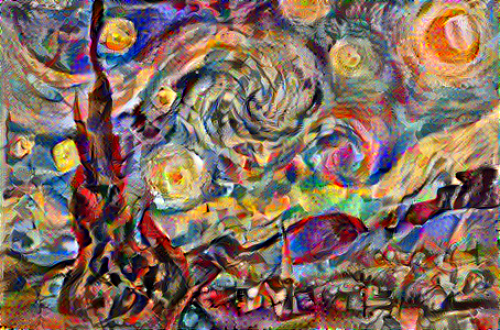
This is an interesting part because we are creating a styled image here. we have defined the number of epochs and steps per epochs and for every epoch, we are calculating loss and optimizing our output image using adam optimizer.
Finally, at last, we are saving output image into the disk, now its time to show off this image to your friends. Play with it and share exciting results.
Below is the demo video showing style transfer in action.
In the next part, we will be using another style transfer technique which will be 100 times faster than this and can be used to style videos too.
Thanks for reading. ✌✌✌